Creating a custom cover

This example will go over the API for creating a custom cover scheme. We will be implementing the epsilon nets outlined in https://arxiv.org/abs/1901.07410. This is meant to illustrate the expected api, not much thought was put into the actual implementation of the cover itself and there may be better ways.

Representing a cover

Zen Mapper represents sets as numpy arrays of indices into a data array. That is to say np.array([1, 2, 5]) represents the set with elements 1, 2, and 5 from the original, high dimensional data. Zen mapper then represents a cover as an Iterable of these cover elements. If you’re not comfortable with what an Iterable is, you can think of them as a list for now. To construct a cover that zen mapper understands will require us to adhere to this format.

Constructing an epsilon net

An epsilon-net is a collection of balls of radius epsilon. The covers used in ball mapper are all variations on generating an epsilon-net. So to start we will focus on creating a function which takes a description of an epsilon-net along with some data and constructs a cover as outlined in the previous section.

import numpy as np


def epsilon_net(centers, epsilon, data) -> list[np.ndarray]:
    if len(data.shape) == 1:
        data.reshape(-1, 1)

    cover = []
    for center in centers:
        # Create a new cover element for each center point
        cover_element = []

        for i, datum in enumerate(data):
            # Check if the distance between the center point
            # and the data point is less than epsilon
            if np.sum((center - datum) ** 2) < epsilon**2:
                # If so append it to our cover element
                cover_element.append(i)

        # Finally add our cover element to the result
        cover.append(np.array(cover_element, dtype=int))

    return cover

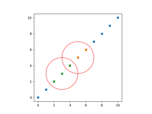
It is worth noting that list[numpy.ndarray] is an Iterable and so is understood by zen mapper. We can then visualize that this cover acts as we hope it would.

import matplotlib.pyplot as plt

# We construct a diagonal dataset
data = np.c_[np.arange(11), np.arange(11)]
centers = np.array([[5, 5], [3, 3]])
epsilon = 2

ax = plt.gca()

# Plot the dataset
ax.scatter(data[:, 0], data[:, 1])

# Compute the cover
cover = epsilon_net(centers, epsilon, data)

# Plot each element of that cover
for i, element in enumerate(cover):
    ax.scatter(
        data[element, 0],
        data[element, 1],
        label=f"Cover Element {i}",
    )

# Visualize each epsilon ball
for center in centers:
    circ = plt.Circle(center, epsilon, color="r", fill=False)
    ax.add_patch(circ)

ax.set_aspect("equal")
ax.legend()
plt.show()

A greedy epsilon net

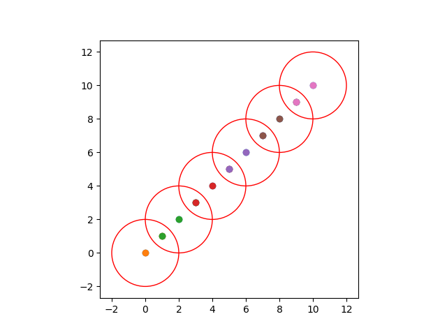
Ball mapper goes on to define a “greedy” epsilon net. The user specifies a dataset and an epsilon value and from there the algorithm proceeds to repeatedly choose a point not currently covered by the epsilon net and adds this point as a center point to the net. We will define a function which implements this algorithm.

def greedy_epsilon_net(epsilon: float, data: np.ndarray):
    # These are the points which are not covered
    to_cover = set(range(len(data)))

    centers = []

    # If there are still points to cover
    while to_cover:
        # Pick the first one in the set
        new_center = to_cover.pop()

        # Add it to the list of centers
        centers.append(data[new_center])
        covered = set()

        for point in to_cover:
            # Mark the point as covered
            if np.sum((data[new_center] - data[point]) ** 2) < epsilon**2:
                covered.add(point)

        # Remove all the points we covered from the set to cover
        to_cover -= covered

    # Construct the cover from these center points
    cover = epsilon_net(centers, epsilon, data)

    # Return the cover along with the centers
    return cover, centers

By returning the center points along with the cover we allow users to introspect how the cover was constructed. We can then visualize the covering scheme in much the same way we visualized the cover.

data = np.c_[np.arange(11), np.arange(11)]
cover, centers = greedy_epsilon_net(epsilon=2, data=data)

ax = plt.gca()
ax.scatter(data[:, 0], data[:, 1])

for element in cover:
    ax.scatter(data[element, 0], data[element, 1])

for center in centers:
    circ = plt.Circle(center, epsilon, color="r", fill=False)
    ax.add_patch(circ)

ax.set_aspect("equal")
plt.show()

Using with mapper

Now that we have a cover we will demonstrate how to plug it into zen mapper to duplicate the analysis done in the original paper. We will be using a similar window dataset to the one they used. We start by generating our data.

def window(num_samples: int) -> np.ndarray:
    data = np.random.rand(num_samples, 2)
    data[:, 1] *= 9
    data[:, 0] += 4 * np.random.randint(0, 3, size=num_samples)
    choice = np.random.randint(0, 2, size=(num_samples, 1))
    return choice * data + (1 - choice) * data[:, [1, 0]]


np.random.seed(42)
data = window(1000)
plt.scatter(data[:, 0], data[:, 1])
plt.gca().set_aspect("equal")
plt.show()

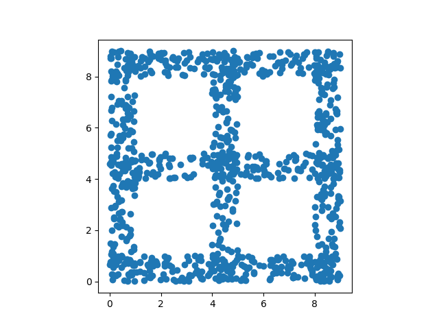
We then can fit our cover to this data set, visualizing it as we did in previous examples

epsilon = 1.25
cover, centers = greedy_epsilon_net(data=data, epsilon=epsilon)

ax = plt.gca()
ax.scatter(data[:, 0], data[:, 1])

for element in cover:
    ax.scatter(data[element, 0], data[element, 1])

for center in centers:
    circ = plt.Circle(center, epsilon, color="r", fill=False)
    ax.add_patch(circ)

ax.set_aspect("equal")
plt.show()

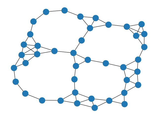
Finally we need to define a clustering algorithm. In this paper they don’t actually cluster anything, instead any datapoint in the ball is deemed to be connected. So we define the following trivial clusterer. See Creating a custom clusterer for more information on how to construct a clusterer for zen mapper.

def trivial(data: np.ndarray, elements: np.ndarray):
    return [np.arange(elements.size)], None

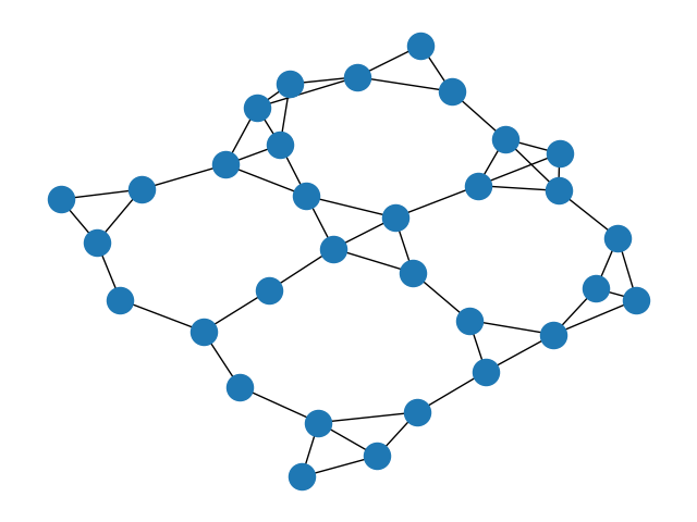
With this we are able to call mapper and get a very similar graph to the one from the paper.

import networkx as nx

import zen_mapper as zm

result = zm.mapper(
    data=data,
    cover=cover,
    clusterer=trivial,
    dim=1,
)

g = zm.to_networkx(result.nerve)
nx.draw_kamada_kawai(g)
plt.show()