Extracting Data from Nodes

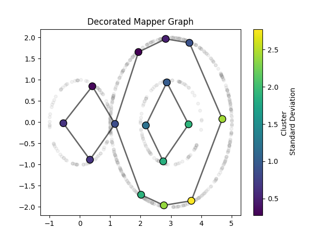
In this example we overlay a resulting mapper graph on top of the scatter-plot of datapoints. The nodes will be placed at the mean of the corresponding cluster. The color of the node will correspond to the standard deviation.

Generate Data

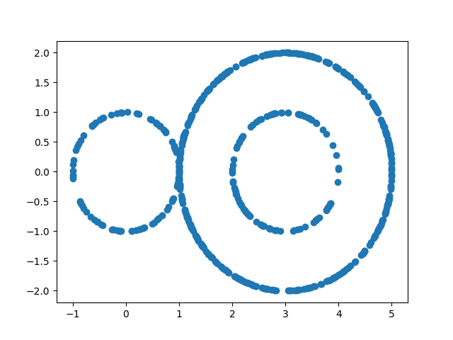
Here we will use sphere generator from kaiju mapper to generate a dataset

import matplotlib.pyplot as plt
import numpy as np
from kaiju_mapper.datasets import sphere

rng = np.random.default_rng(123)

circles = (
    sphere(dim=1, num_samples=100, seed=rng),
    sphere(dim=1, num_samples=400, radius=2, center=(3, 0), seed=rng),
    sphere(dim=1, num_samples=100, radius=1, center=(3, 0), seed=rng),
)

data = np.vstack(circles)

plt.scatter(data[:, 0], data[:, 1])
plt.show()

Implement Mapper

from sklearn.cluster import DBSCAN

import zen_mapper as zm

cover_scheme = zm.Width_Balanced_Cover(n_elements=7, percent_overlap=0.2)
projection = data[:, 0]
clusterer = zm.sk_learn(DBSCAN(eps=0.5))

result = zm.mapper(
    data=data,
    projection=projection,
    clusterer=clusterer,
    cover_scheme=cover_scheme,
    dim=1,
)

Accessing Data Points from Nodes

The MapperResult.nodes attribute holds a list of clusters which are each a list of data indices belonging to the cluster. Once you have access to these indices you can run your own analysis.

cluster_centers = []
cluster_stds = []

# Get data from nodes!
for data_indices in result.nodes:
    # This is where we extract data
    cluster_points = data[data_indices]
    center = np.mean(cluster_points, axis=0)
    std = np.std(cluster_points)
    cluster_centers.append(center)
    cluster_stds.append(std)

node_positions = np.array(cluster_centers)
node_stds = np.array(cluster_stds)

Visualize

We can access all k-simplices by calling the MapperResult.nerve[k] attribute. This will return simplices stored as a (k+1)-tuple of node_ids. One can then apply the same process as above to access the corresponding data points for analysis/visualization. For now, we will just use this to draw edges manually.

plt.scatter(data[:, 0], data[:, 1], alpha=0.1, c="gray", s=20)

# draw edges from nerve attribute
for node1_id, node2_id in result.nerve[1]:
    x_coords = [node_positions[node1_id, 0], node_positions[node2_id, 0]]
    y_coords = [node_positions[node1_id, 1], node_positions[node2_id, 1]]
    plt.plot(x_coords, y_coords, "k-", alpha=0.6, linewidth=2)

# draw nodes
scatter = plt.scatter(
    node_positions[:, 0],
    node_positions[:, 1],
    c=node_stds,
    s=100,
    cmap="viridis",
    edgecolors="black",
    linewidth=1,
    zorder=2,  # just places nodes above edges
)

plt.colorbar(scatter, label="Cluster \n Standard Deviation")
plt.title("Decorated Mapper Graph")
plt.show()